
Worksheet Graphing Exponential Functions offers a powerful way to deepen students’ grasp of how exponential relationships behave visually, providing hands‑on practice that translates theory into tangible skills. In this guide, we walk through the fundamentals, common pitfalls, and practical techniques that make these worksheets a reliable tool for both teachers and learners.
Understanding Exponential Functions

What Is an Exponential Function?
An exponential function follows the general form y = a · bx, where a is the initial value (often called the y‑intercept), and b is the base that determines the rate of growth or decay. When b > 1, the function grows rapidly; when 0 < b < 1, it declines toward zero.
Key Differences From Polynomial Functions
Unlike linear or polynomial functions, exponential functions:
- Show no turning points—curves are always monotonic.
- Have a horizontal asymptote at y = 0 (for growth) or y = 0 (for decay).
- Grow or shrink by a consistent factor for each unit increase in x.
Key Features of Exponential Graphs

Asymptotes and Intercepts
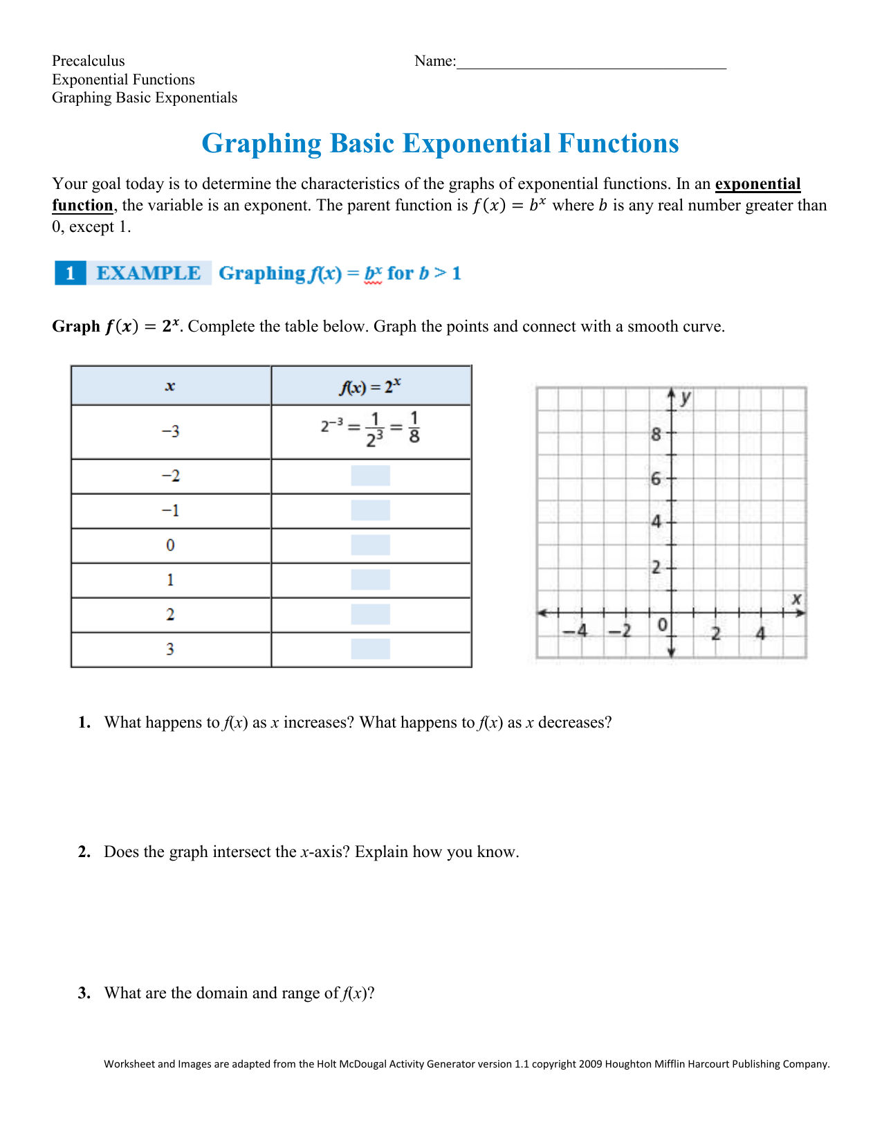
Every exponential graph has a horizontal asymptote at y = 0. The y‑intercept is simply the value of a, occurring when x = 0. Students should identify these points first to anchor the rest of the plot.
Growth vs. Decay Patterns
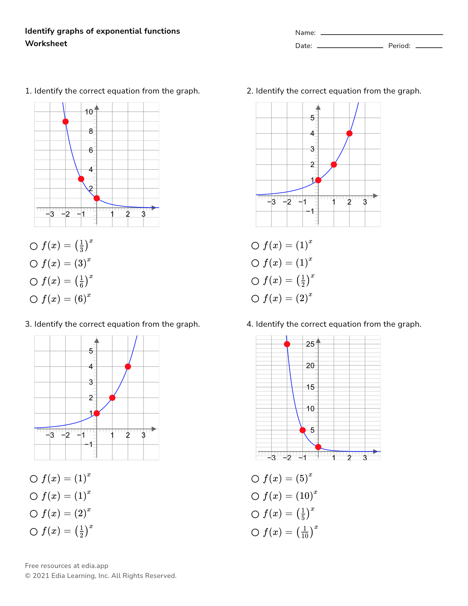
When b > 1, the graph rises steeply as x increases. When 0 < b < 1, the graph declines, approaching the asymptote without ever touching it. Recognizing the base’s magnitude helps predict the shape before sketching.
Scaling and Shifting
Multiplying by a constant scales the graph vertically, while adding a constant to x shifts it horizontally. Worksheets often ask for transformations; mastering these concepts is essential for accurate graphing.
Common Worksheet Questions and How to Approach Them

Identifying the Base and Coefficient
Most problems present the function in standard form, but some use alternative expressions, such as y = 3 · 2–x. Encourage students to rewrite the expression to isolate the base and coefficient clearly.
Calculating Key Points
Students should calculate at least three points: the y‑intercept, a point where x = 1, and a point where x = –1 (if defined). These anchor the curve and allow for accurate plotting.
Recognizing Transformations
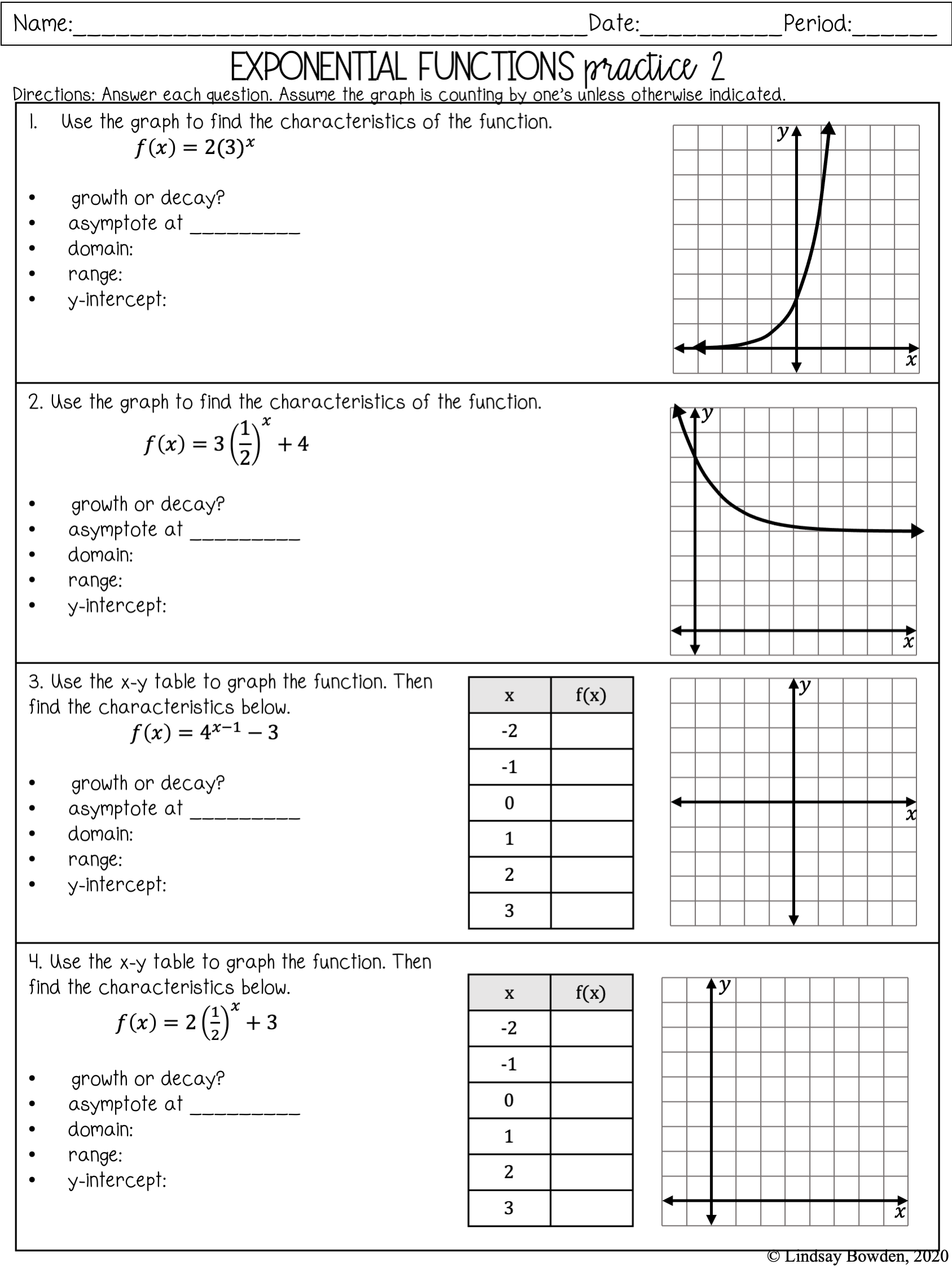
When the function is altered, such as y = 4 · (0.5)x–2 + 1, identify each transformation step: horizontal shift right by 2, vertical stretch by 4, and vertical shift up by 1. Breaking it into components keeps the graphing process organized.
Step‑by‑Step Guide to Graphing Exponential Functions

Step 1: Determine the Function Type
Check if the base is greater than 1 for growth or between 0 and 1 for decay. This informs the overall direction of the curve.
Step 2: Identify the Asymptote
Draw a dashed horizontal line at y = 0 unless the function includes a vertical shift that changes the asymptote’s location.
Step 3: Plot the Y‑Intercept
Plug x = 0 into the function. Mark this point accurately; it often provides a convenient anchor.
Step 4: Compute Additional Points
- For growth: Evaluate at x = 1 and x = 2 to see how quickly the curve rises.
- For decay: Evaluate at x = –1 and x = –2 to observe the approach toward the asymptote.
Step 5: Apply Transformations
Use the transformation checklist: horizontal shift, vertical stretch/compression, and vertical shift. Update the coordinates accordingly before plotting.
Step 6: Sketch the Curve
Connect the plotted points smoothly, respecting the asymptote and ensuring the curve never crosses it. Remember that exponential growth curves accelerate, while decay curves flatten out.
Step 7: Verify Accuracy
Check that the graph aligns with the calculated points and that asymptotic behavior matches the theoretical expectation.
Real-World Applications
Population Growth
Biological populations often follow exponential growth. By graphing P(t) = P0 · ert, students can visualize how populations expand over time and understand carrying capacity limits.
Radioactive Decay
Physics students model decay with functions like N(t) = N0 · (1/2)t/T½. Plotting this shows the half-life process, reinforcing the concept of exponential decline.
Compound Interest
Finance teachers use A = P · (1 + r)n to illustrate how money grows with continuous compounding. Students can compare growth curves for different rates to appreciate the power of exponential increases.
Tips for Students
Use a Graphing Calculator Strategically
While calculators can plot points instantly, rely on them to confirm your manual work rather than as the primary tool. The mental exercise of determining key points solidifies understanding.
Practice with Variations
Mix growth and decay problems, include horizontal shifts, and vary coefficients. The more diverse the practice, the better students become at spotting patterns.
Keep a Transformation Cheat Sheet
Create a quick reference that lists how each transformation affects the graph. Having this at hand reduces mistakes during timed worksheets.
Peer Review Sessions
Exchange completed worksheets with classmates. Reviewing each other’s graphs can highlight common mistakes and reinforce correct techniques.
Frequently Asked Questions
Why does the graph never cross the asymptote?
Because exponential functions approach the asymptote asymptotically; the distance between the curve and the line decreases but never reaches zero. This is a defining property of the function.
Can an exponential function have a vertical asymptote?
Not in the standard form y = a · bx. Vertical asymptotes arise in rational functions, not pure exponentials.
What if the base is negative?
Standard exponential functions require a positive base to maintain continuity over real numbers. Negative bases produce complex outputs for non‑integer exponents, which is beyond typical worksheet scope.
Final Thoughts

Mastering Worksheet Graphing Exponential Functions equips students with a robust visual toolkit for understanding growth and decay. By systematically identifying function types, calculating key points, applying transformations, and verifying asymptotic behavior, learners gain confidence that translates into higher‑order problem solving across mathematics, science, and economics. Consistent practice, coupled with real‑world examples, turns abstract equations into intuitive, memorable concepts—an essential foundation for any aspiring mathematician or analyst.


